Integration
We provide a variety of non-linear equations used for testing numerical integration algorithms.
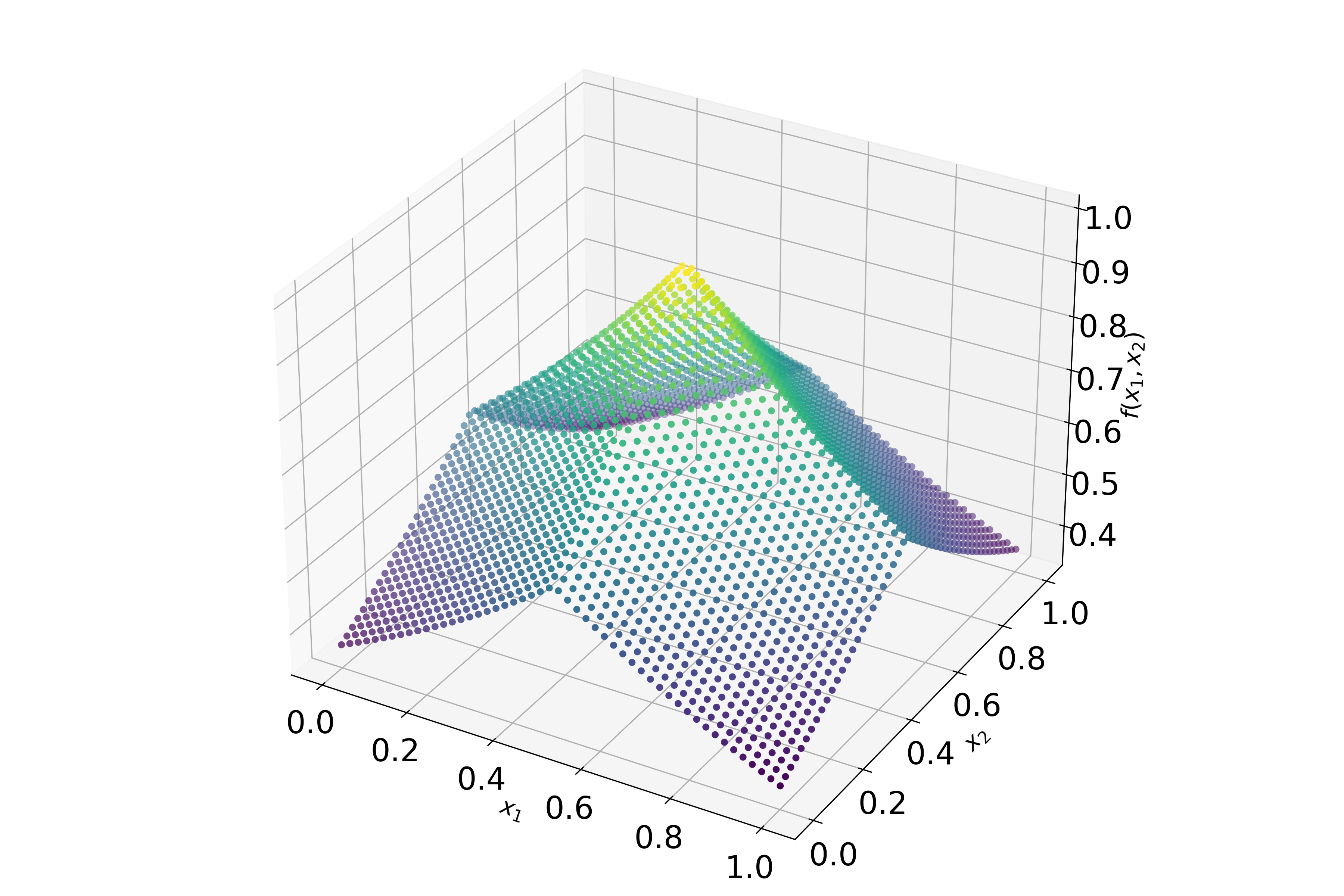
- temfpy.integration.continuous(x, u, a)[source]
Continuous Integrand Family.
\[f(x)=\exp{\left(-\sum_{i=1}^p a_i \mid x_i -u_i \mid \right)}\]- Parameters
x (array_like) – Input domain with dimension \(p\) and \(x \in [0,1]^p\).
u (array_like) – Location vector with dimension \(p\) and \(u \in [0,1]^p\).
a (array_like) – Weight vector with dimension \(p\).
- Returns
Output domain
- Return type
float
Notes
This function was proposed by Alan Genz in [G1984]. It can be integrated analytically quickly with high precision. Evaluated at two dimensions, the function has a flat surface and one peak close to the centre of the integration region. Large values in the location vector \(a\) result in a sharp peak and a more difficult integration.
References
- G1984
Genz, A. (1984). Testing multidimensional integration routines. In Proc. of international conference on tools, methods and languages for scientific and engineering computation (pp. 81-94). Elsevier North-Holland.
Examples
>>> import numpy as np
>>> from temfpy.integration import continuous
>>>
>>> p = np.random.randint(1,20)
>>> x = np.repeat(0.5,p)
>>> u = x
>>> a = np.repeat(5,p)
>>> np.allclose(continuous(x,u,a), 1)
True
- temfpy.integration.corner_peak(x, a)[source]
Corner Peak Integrand Family.
\[f(x)=\left(1 + \sum_{i=1}^p a_i x_i \right)^{p+1}\]- Parameters
x (array_like) – Input domain with dimension \(p\) and \(x \in [0,1]^p\).
a (array_like) – Weight vector with dimension \(p\).
- Returns
Output domain
- Return type
float
Notes
This function was proposed by Alan Genz in [G1984]. It can be integrated analytically quickly with high precision. Evaluated at two dimensions, the function has a flat surface and a single sharp peak in one corner of the integration region. Large values in the location vector \(a\) result in a sharper peak and a more difficult integration.
References
- G1984
Genz, A. (1984). Testing multidimensional integration routines. In Proc. of international conference on tools, methods and languages for scientific and engineering computation (pp. 81-94). Elsevier North-Holland.
Examples
>>> import numpy as np
>>> from temfpy.integration import corner_peak
>>>
>>> p = np.random.randint(1,20)
>>> x = np.repeat(0,p)
>>> a = np.repeat(5,p)
>>> np.allclose(corner_peak(x,a), 1)
True
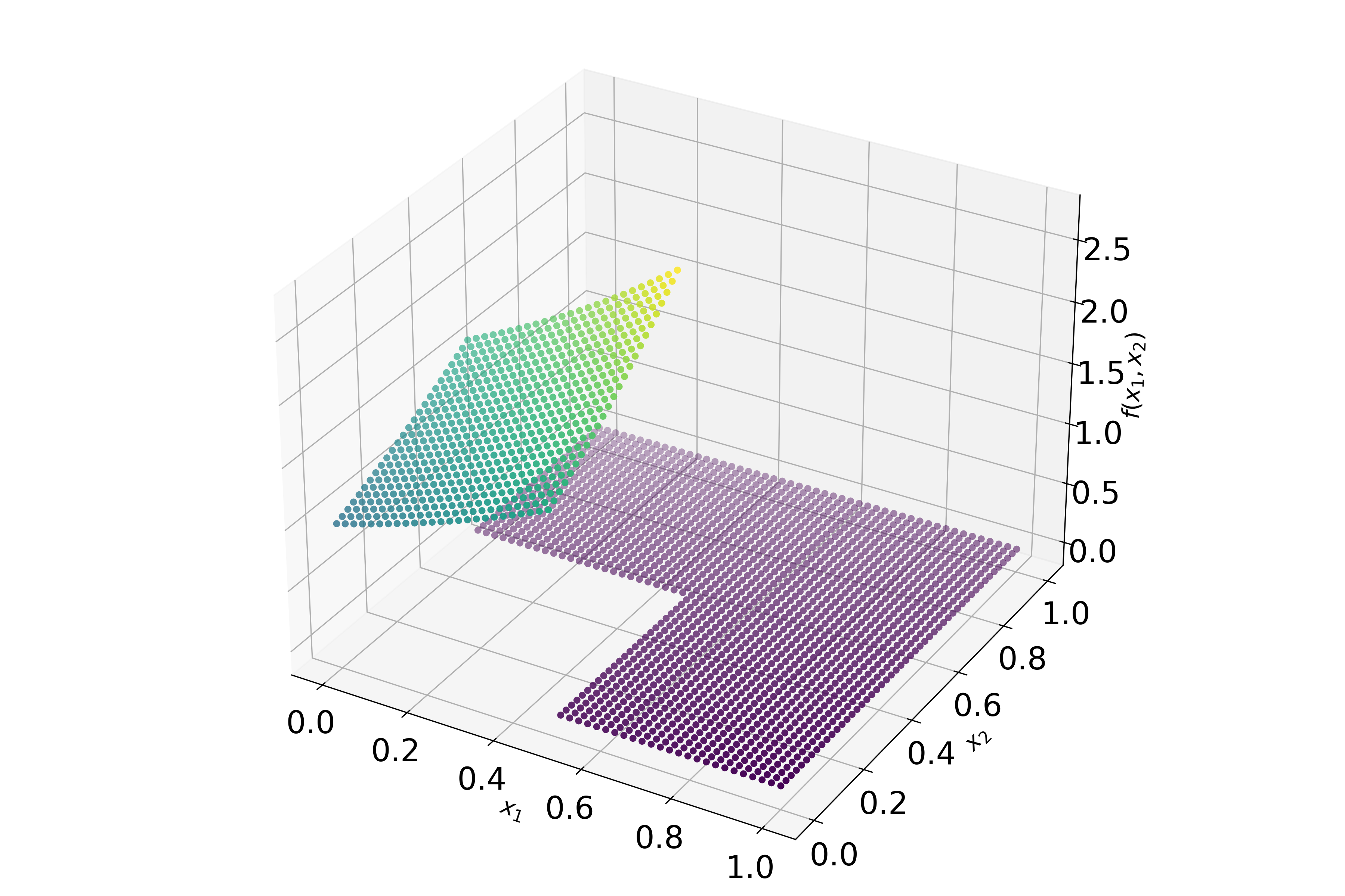
- temfpy.integration.discontinuous(x, u, a)[source]
Discontinuous Integrand Family.
\[\begin{split}f(x) = \begin{cases} 0, & x_1 > u_1 \text{ or } x_2 > u_2 \\ \exp{\left(\sum_{i=1}^p a_i x_i \right)}, & \text{otherwise} \end{cases}\end{split}\]- Parameters
x (array_like) – Input domain with dimension \(p\) and \(x \in [0,1]^p\).
u (array_like) – Location vector with dimension \(1\), if \(p = 1\), and with dimension \(2\), if \(p > 1\), that determines in which area the function is equal to zero.
a (array_like) – Weight vector with dimension \(p\).
- Returns
Output domain
- Return type
float
Notes
This function was proposed by Alan Genz in [G1984]. It can be integrated analytically quickly with high precision. Evaluated at two dimensions, the function has one peak close to the centre of the integration region and is flat at zero for greater values, as specified in \(u\). Large values in the location vector \(a\) result in a sharp peak and a more difficult integration.
References
- G1984
Genz, A. (1984). Testing multidimensional integration routines. In Proc. of international conference on tools, methods and languages for scientific and engineering computation (pp. 81-94). Elsevier North-Holland.
Examples
>>> import numpy as np
>>> from temfpy.integration import discontinuous
>>>
>>> p = np.random.randint(1,20)
>>> x = np.repeat(0,p)
>>> u = [0.5,0.5]
>>> a = np.repeat(5,p)
>>> np.allclose(discontinuous(x,u,a), 1)
True
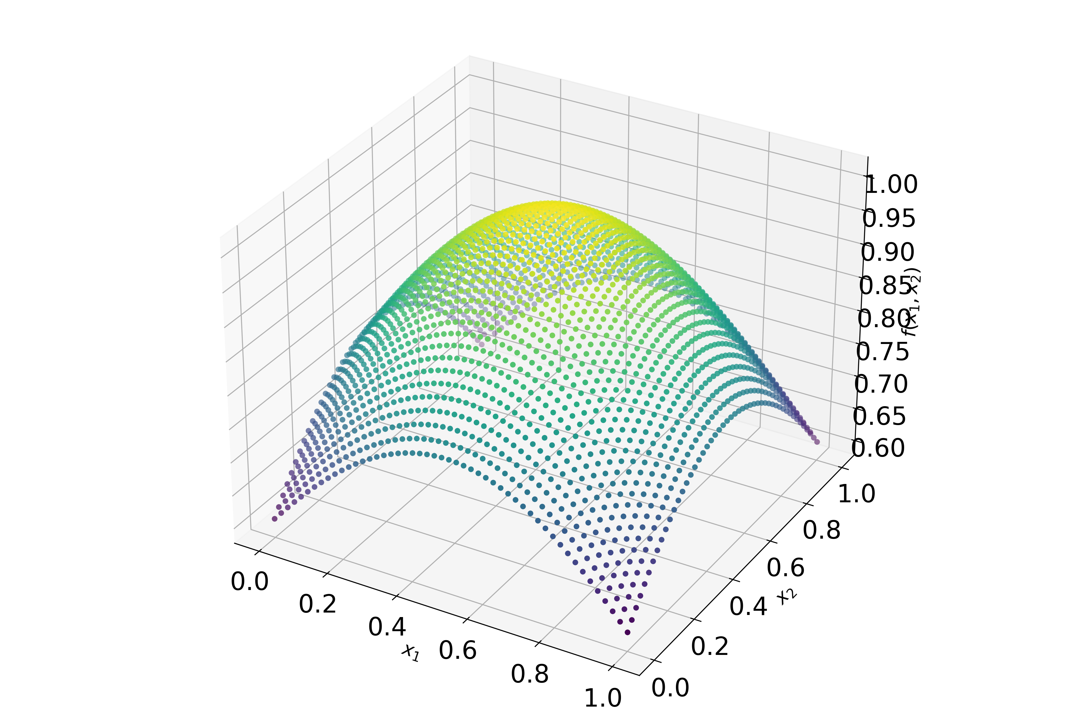
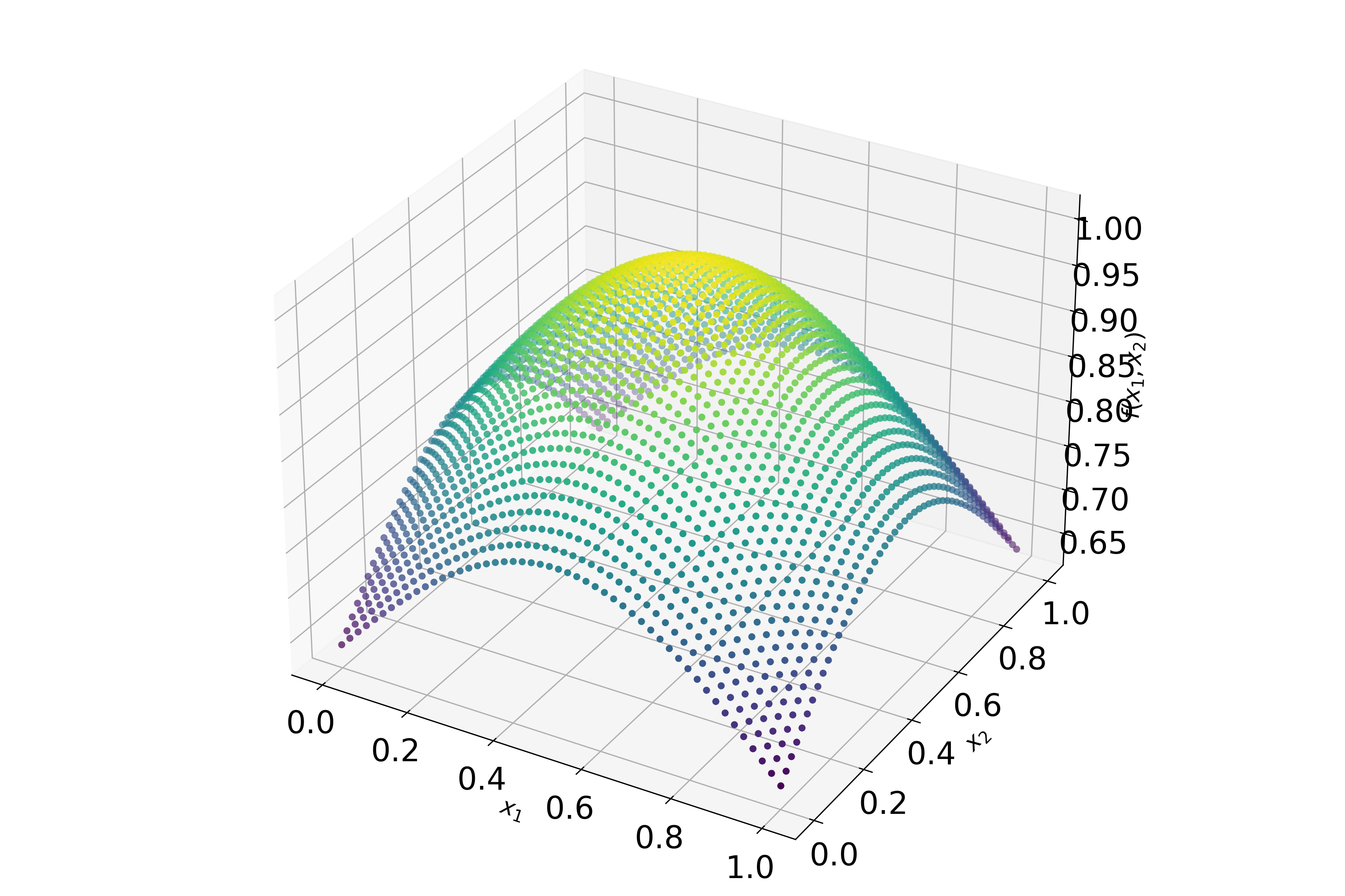
- temfpy.integration.gaussian_peak(x, u, a)[source]
Gaussian peak Integrand Family.
\[f(x)=\exp{\left(-\sum_{i=1}^p a_i^2 (x_i -u_i)^2 \right)}\]- Parameters
x (array_like) – Input domain with dimension \(p\) and \(x \in [0,1]^p\).
u (array_like) – Location vector with dimension \(p\) and \(u \in [0,1]^p\).
a (array_like) – Weight vector with dimension \(p\).
- Returns
Output domain
- Return type
float
Notes
This function was proposed by Alan Genz in [G1984]. It can be integrated analytically quickly with high precision. Evaluated at two dimensions, the function has a Gaussian peak close to the centre of the integration region. Large values in the location vector \(a\) result in a sharp peak and a more difficult integration.
References
- G1984
Genz, A. (1984). Testing multidimensional integration routines. In Proc. of international conference on tools, methods and languages for scientific and engineering computation (pp. 81-94). Elsevier North-Holland.
Examples
>>> import numpy as np
>>> from temfpy.integration import gaussian_peak
>>>
>>> p = np.random.randint(1,20)
>>> x = np.repeat(0.5,p)
>>> u = x
>>> a = np.repeat(5,p)
>>> np.allclose(gaussian_peak(x,u,a), 1)
True
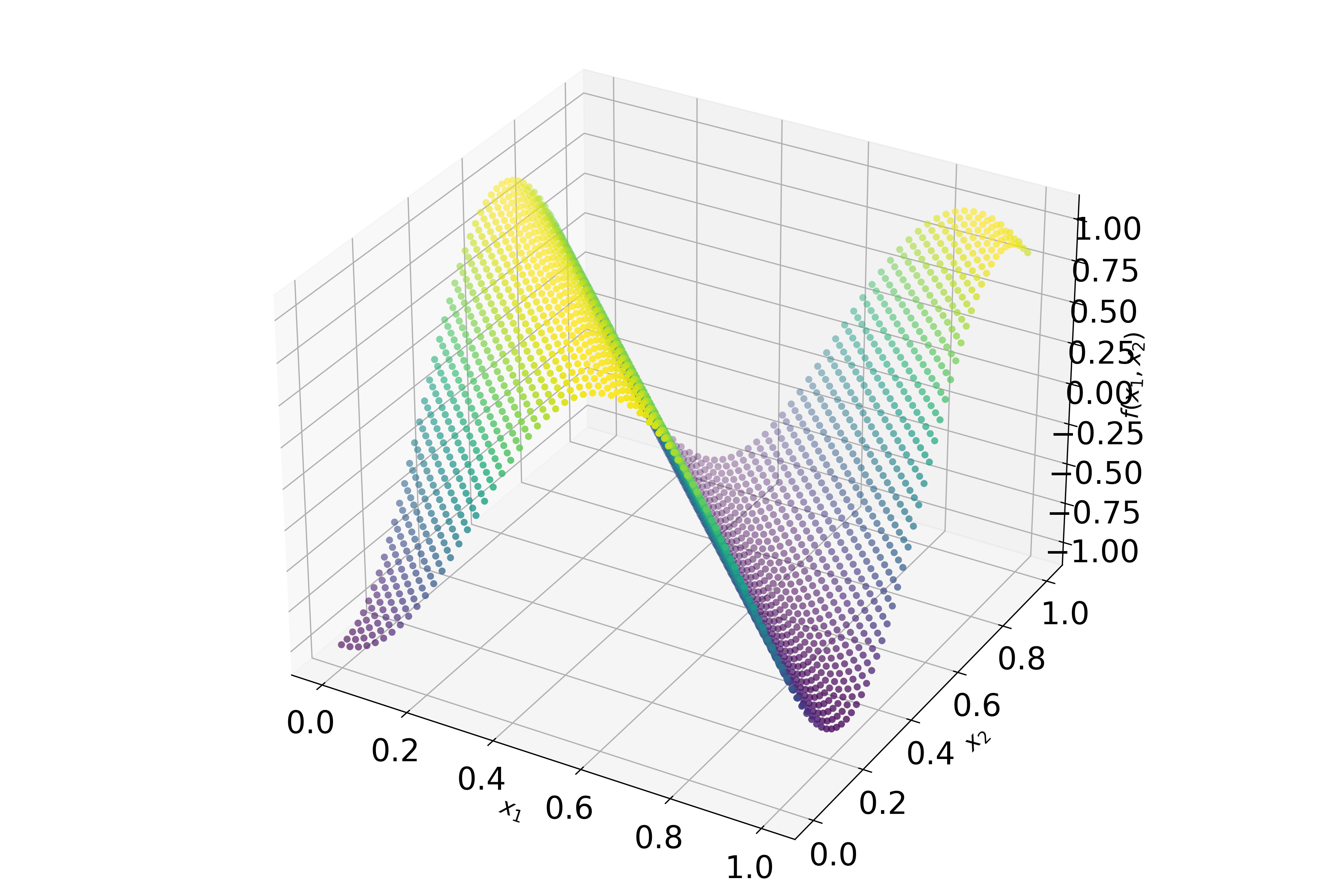
- temfpy.integration.oscillatory(x, a, b)[source]
Oscillatory Integrand Family.
\[f(x)= \cos\left(2 \pi b + \sum_{i=1}^p a_i x_i \right)\]- Parameters
x (array_like) – Input domain with dimension \(p\) and \(x \in [0,1]^p\).
a (array_like) – Weight vector with dimension \(p\).
b (int) – Scale value that influences the location of the oscillatory.
- Returns
Output domain
- Return type
float
Notes
This function was proposed by Alan Genz in [G1984]. It can be integrated analytically quickly with high precision. Large values in the location vector \(a\) result in a higher frequency of oscillations and a more difficult integration.
References
- G1984
Genz, A. (1984). Testing multidimensional integration routines. In Proc. of international conference on tools, methods and languages for scientific and engineering computation (pp. 81-94). Elsevier North-Holland.
Examples
>>> import numpy as np
>>> from temfpy.integration import oscillatory
>>>
>>> p = np.random.randint(1,20)
>>> x = np.repeat(np.pi/4,p)
>>> a = np.repeat(-6/p,p)
>>> b = 1
>>> np.allclose(oscillatory(x,a,b), 0)
True
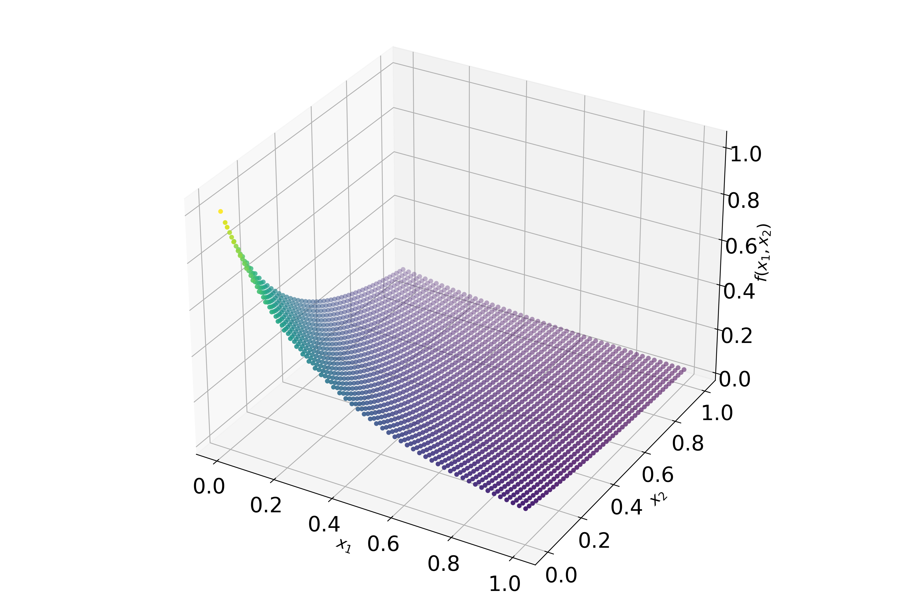
- temfpy.integration.product(x, u, a)[source]
Product Peak Integrand Family.
\[f(x)=\prod \frac{1}{\sum_{i=1}^p a_i^{-2} (x_i -u_i)^2}\]- Parameters
x (array_like) – Input domain with dimension \(p\) and \(x \in [0,1]^p\).
u (array_like) – Location vector with dimension \(p\) and \(u \in [0,1]^p\).
a (array_like) – Weight vector with dimension \(p\).
- Returns
Output domain
- Return type
float
Notes
This function was proposed by Alan Genz in [G1984]. It can be integrated analytically quickly with high precision. Evaluated at two dimensions, the function has a peak in the centre of the integration region. Large values in the location vector \(a\) result in a larger peak and a more difficult integration.
References
- G1984
Genz, A. (1984). Testing multidimensional integration routines. In Proc. of international conference on tools, methods and languages for scientific and engineering computation (pp. 81-94). Elsevier North-Holland.
Examples
>>> import numpy as np
>>> from temfpy.integration import product
>>>
>>> p = np.random.randint(1,20)
>>> x = np.repeat(0.5,p)
>>> u = x
>>> a = np.repeat(1,p)
>>> np.allclose(product(x,u,a), 1)
True